| Hermetic Word Frequency Counter Advanced Version |
| Zipf's Law |
Use of this Program to Illustrate Zipf's Law
Zipf's Law is a statement based on observation rather than theory. It is often true of a collection of instances of classes, e.g., occurrences of words in a document. It says that the frequency of occurrence of an instance of a class is roughly inversely proportional to the rank of that class in the frequency list.More exactly, suppose a word occurs f times and that in the list of word frequencies it has a certain rank, r. Then if Zipf's Law holds we have (for all words) f = a/rb where a and b are constants and b is close to 1.
Taking the logarithm of each side of the equation we obtain log(f) = log(a) - b*log(r). (The log function can be to any base, such as e or 10.) Thus if Zipf's law holds of a particular collection then if we graph log(f) against log(r) the graph will be a straight line with slope close to -1.
A consequence is that (if b = 1) a word of rank k occurs 1/kth as often as the most-frequently-occurring word. We see this from: f(k)/f(1) = (a/k)/(a/1) = 1/k. And for every k occurrences of a word of rank j there are approximately j occurrences of a word of rank k.
Since the Advanced Version (but not the basic version) will output a table of frequencies and ranks, it can be used (with the help of a spreadsheet such as Excel) to illustrate Zipf's Law, and to test particular collections of words as to how closely Zipf's law is true of them. Two examples will now be given.
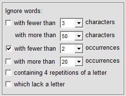
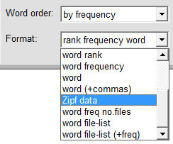 Start the program and in the 'Settings' window click on 'Restore defaults', then check/uncheck the checkboxes as shown at left. If a common words file is specified then clear the file name (this is so that the common words, such as 'of' and 'in' will be counted). Select 'by frequency' for word order, and 'Zipf data' for display format. If the software has been activated then specify an output file, e.g. 'output.txt'.
Select 'Single file' as the source of the text, and as the input file specify any text file consisting of natural language. In the first example we use the file oil_bourse.txt (15,374 bytes), which can be downloaded from this site as oil_bourse.zip. Click on 'Count words/phrases' then on 'Count all words'. At the end of the operation the Zipf data will have been written to output.txt and the screen will look like this:
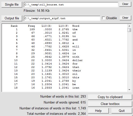
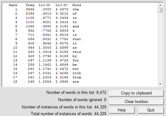
The L10(R) and L10(F) values are the logarithm (to the base 10) of the rank values and the frequency values respectively. The 615 "ignored" words are those that occur only once.
We now wish to plot the log values, which can be done in Excel. Open the output file output.txt in Excel (remember that it is a text file, not an .xls file). Select 'Delimited' and click on 'Next'; check 'Tab' and click on 'Next'; click 'Finish'. Highlight the two columns of log values, beginning with the data from the cells immediately below L10(R) and L10(F). Then click on the icon for the Chart Wizard, select 'XY (Scatter)', with data points connected by lines. After adding a title and labeling the two axes of the graph we eventually obtain the following:
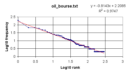
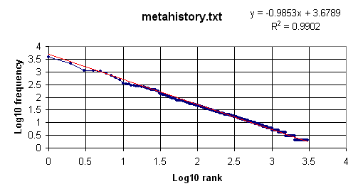
Clearly the log-log plot is roughly linear, confirming a Zipf distribution, although the slope is -0.8143, a little larger than the Zipfian ideal of -1.
For the second example we use the file metahistory.txt (272,196 bytes), which can be downloaded from this site as metahistory.zip. At the end of the operation (it takes about 12 seconds) the Zipf data will have been written to output.txt and the screen will look like this:
Repeating the procedure described above we arrive at this graph:
In contrast, a 2 MB file containing over 100,000 words randomly generated, although it produced a linear fit, did so with a slope of about -0.3, far from the Zipfian -1.
| Introduction | User Manual: Contents |
| Hermetic Systems Home Page | |